

TU Delft experiment - Persistent Current Qubit
We studied the coherent time evolution between the two quantum states of a 3 Josephson junction superconducting flux-qubit. The superposition of the two states carrying opposite macroscopic persistent currents is manipulated by resonant microwave pulses. Readout by means of switching-event measurement with an attached superconducting quantum interference device revealed quantum-state oscillations with high fidelity. Under strong microwave driving it was possible to induce hundreds of coherent oscillations. Pulsed operations on this first sample yielded a relaxation time of 900 ns and a free-induction dephasing time of 20 ns. These results are promising for future solid-state quantum computing.The qubit and the on-chip environment
The sample fabrication is done by means of e-beam lithography and metal evaporation using the nanotechnology facilities located in our campus (DIMES, TU Delft). The central part of the circuit is shown in Fig. 1A. The evaporation of Al from two different angles (shadow evaporation) with an oxidation process in-between gives the small overlapping regions that form the Josephson junctions. The three in-line Josephson junctions together with the small loop defines the qubit in which the persistent current can flow in two directions, as shown by the arrows. The middle junction of the qubit is α=0.8 times smaller than the other two and the ratio of qubit/SQUID areas is about 1:3. The critical current of SQUID junctions is ~2.2 µA whereas the critical current of the qubit largest junction is ~0.5 µA.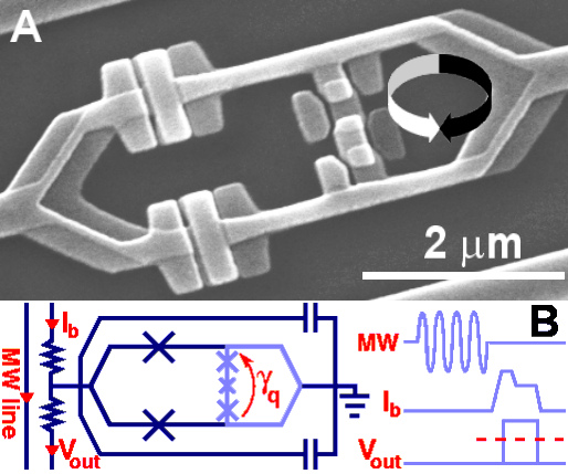
Fig. 1 (A) Scanning electron micrograph of a flux-qubit (small loop with 3 Josephson junctions) and the attached DC-SQUID (large loop with two big Josephson junctions). Arrows indicate the two directions of the persistent current in the qubit. (B) Schematic of the on-chip circuit; crosses represent the Josephson junctions.
The SQUID is shunted by two on-chip capacitors (~5 pF each) to reduce the SQUID plasma frequency and biased through a resistor (~150 Ω, on-chip) to avoid parasitic resonances in the leads. Symmetry of the circuit is introduced to suppress excitation of the SQUID from the qubit-control pulses (see Fig. 1B). The microwave (MW) line provides microwave current bursts inducing oscillating magnetic fields in the qubit loop. The current line provides the measuring pulse Ib and the voltage line allows the readout of the switching pulse Vout. The Vout signal is amplified and a threshold discriminator (dashed line) detects the switching event at room temperature. The sample is enclosed in a gold-plated copper shielding box mounted onto the mixing chamber of our fridge.
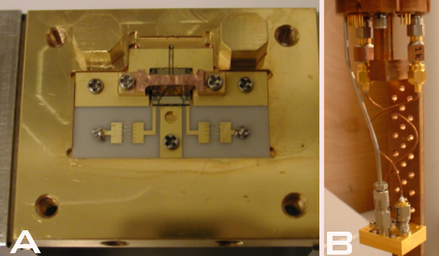
Fig. 2 (A) Copper shielding cavity platted with gold. Under the fixing clamp one can see the chip containing the MW waveguide, capacitors, resistors and the superconducting SQUID-qubit device. (B) The cavity is closed and then mounted on the cold-finger of the mixing chamber.
The qubit: an artificial two-level system
The qubit energy levels as a function of the superconductor phase γq across the junctions (Fig. 1B) are determined by the charging energy EC=e2/2C and the Josephson energy EJ= hIC/4πe of the qubit outer junctions (IC and C are their critical current and capacitance) together with the α ratio (in Fig. 4A one can see the first three levels computed by numerical diagonalization).At our operating temperatures (≈25 mK) and close to γq=π, the qubit behaves like a two-level system as the contribution of the upper levels can be completely neglected. The energy separation can be written as E10 = E1-E0 where E1, E0 are the energies of the eigenstates |0> and |1>. These eigenstates are described by the effective Hamiltonian H=-εσz/2-Δσx/2, where σz,x are the Pauli spin matrices, Δ is the level repulsion, ε≈IpΦ0(γq-π)/π with Ip≈2παEJ/Φ0 the qubit maximum persistent current. The qubit levels resulting from the above Hamiltonian, as well as the corresponding eigenstates, are shown in Fig. 3 (top-half).
The qubit initialization, operation and readout
In the qubit energy diagram (Fig. 3, top) one can note a point of a particular interest: the symmetry point, for ε=0 (no bias) which in our case translates into γq=π. Here, the qubit is insensitive in first order to noise in the bias ε, though measuring the qubit is not possible (a SQUID-based readout would give <σz>=0 for both |0> and |1> states). This simple observation suggests that one should separate the operation and the readout processes by using a bias shift (e.g. as depicted in the Fig. 3) from the symmetry point to a region where <σz0>≠<σz1> .To illustrate the qubit initialization, operation and readout, we will use the well-known Bloch sphere representation (Fig. 3).
[note on the Bloch sphere:
the state of a two-level system in the basis {|↑>,|↓>} can be written as α|↑>+β|↓>. One can than represent the qubit state on a sphere using the spherical coordinates r=1, θ=2tan-1|β/α|, φ=the phase difference between α and β (they are C-numbers!).]
Initialization
The qubit is initialized to the ground state simply by allowing it to relax. To operate the qubit in the optimum conditions, one should apply a magnetic flux through the qubit area of ∼Φ0/2 (or a phase bias) such as γq=π. In Fig.3, the initial state |Q>=|0> is along the qubit axis (defined by the direction of the two eigenstates).Operation
Pulsed microwave excitations are injected on the MW line (Fig.1B) inducing an oscillating magnetic field through the qubit loop. We can control the MW frequency F and the pulse length.
Consequently, the qubit state evolves driven by a time-dependent term (-1/2)εmwcos(2πFt)σz in the Hamiltonian where εmw is the energy-modulation amplitude proportional to the microwave amplitude. This dynamic evolution is similar to that of spins in magnetic resonance. When the MW frequency equals the energy difference of the qubit, the qubit oscillates between the ground state and the excited state. This phenomenon is known as Rabi oscillation. In the frame rotating around the qubit axis with the MW frequency F, the qubit spin precesses around a constant magnetic field ∝εmw (Fig. 3, MW pulse ON). Thus, the Rabi frequency depends linearly on the MW amplitude. The pulse length together with the MW amplitude defines the relative occupancy of the ground and excited state, given by the coefficients α and β in Fig. 3.
Once the MW pulse is turned OFF, the qubit rotates around the qubit axis with the Larmor frequency, E10. To quantify the coherent superposition of the |0> and |1> states, we should measure <σx> (the blue segment in Fig. 3, MW pulse OFF).
Readout
As mentioned previously, a SQUID cannot measure <σx> but only <σz> which would be zero for any α and β at the symmetry point, γq=π. We need a bias shift ε=0 ⇒ ε>0 to reach a region in the qubit spectrum with finite <σz>. In the Bloch sphere representation, this is equivalent with a tilt of the precession cone followed by a measurement of the magenta segment. To preserve the information on the states superposition, this shift has to be adiabatically slow but still much faster than the relaxation time. It turns out that such a shift comes for free, with the readout scheme we proposed in this experiment (the shift is generated by the raise of the Ib pulse, see below).
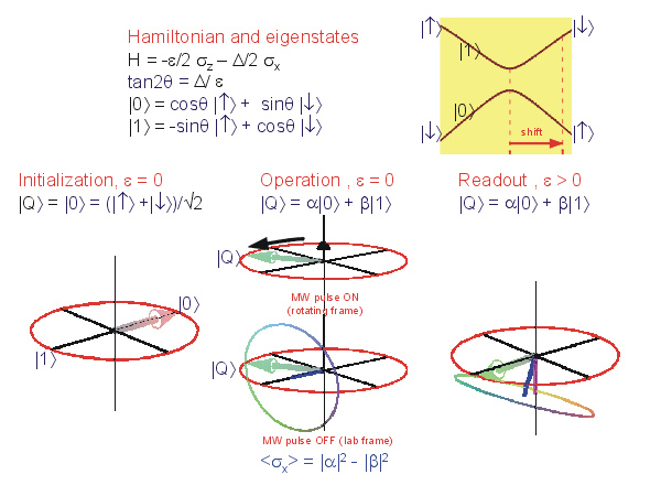
Fig. 3 Top: Qubit Hamiltonian and eigenstates in the two-level system approximation and the corresponding energy levels. Bottom: The initialization, operation and the readout stages, illustrated on the Bloch sphere. The first two are done at the symmetry point whereas the readout first shifts the qubit in a region whith σz0≠σz1, then performs the measurement.
Readout: automatic bias shift and switching event measurements
The readout current pulse is sketched in Fig.1 B. It consists of a short current pulse of length ∼50 ns followed by a trailing plateau of ∼500 ns. During the short pulse, the SQUID either switches to the gap voltage or stays at zero voltage. The trailing plateau is above the retrapping current and keeps alive the switching event (if any) for longer times, to ease our room temperature detection. The switching probability Psw is obtained by repeating the whole sequence of reequilibration, microwave control pulses and readout few thousands times. The switching probability v. Ib gives us also a way to define the notion of switching current: Isw is Ib that gives Psw=50%.When the flux penetrating the qubit area is ∼Φ0/2, the SQUID switching current is close to the 3Φ0/2 minima (remember, the qubit:SQUID area ratio is 1:3). This means that during the qubit operation, a large circulating current is flowing in the SQUID. When the SQUID bias current is switched on, the circulating current changes and the currents in the SQUID arms have no longer opposite values. Due to the shared kinetic and geometric inductances of the joint part, the qubit-SQUID coupling is relatively large (∼9 pH) and consequently, the variation of the SQUID circulating current influences the phase γq across the qubit junctions. By solving a non-linear system of equations formed by the classical current-phase relations and the current conservation laws one gets the amount of the phase shift Δγq generated by the ramp of the bias current. For the parameters of our circuit, we obtain a shift Δγq≈0.01π before the SQUID switching.
It is very important to underline here that the switching of the SQUID occurs for different values of the ramping current Ib (Fig. 1B), depending on the qubit persistent current: Isw0≠Isw1. In this way we can distinguish the state of the qubit, between |0> or |1>. All we have to do is to adjust the height of the Ib pulse between the Isw0,1 values, such as the SQUID switches if the qubit is in one state, for instance |0>, and it doesn't switch if the qubit is in the other state, for instance |1> (in this case Isw0<Ib<Isw1).
[note on the single shot resolution:
If the difference Isw0-Isw1 is sufficiently large to separate the SQUID switching histograms corresponding to the two possible qubit states, the readout reveals single shot resolution. It means that a single switching event can give complete information on the qubit state. However, in real life, one has to integrate a number of switching events to extract this information. ]
Spectroscopy
A first type of experiment one can perform on a two-level system is to examine the energy spectrum by spectroscopic means. In Fig. 4A the qubit energy diagram is calculated for EJ/EC=35, EC=7.4 GHz and α=0.8. One can easily see that the 3rd level (dark gray) is far away from the ground (red) and first excited (green) level in the region of our interest, γq/π∼0.98−1.02 confirming our working hypothesis (two-level system). The average SQUID switching current Isw versus applied flux shows the change of the qubit ground state circulating current (Fig. 4B). Here, the Ib pulse amplitude is adjusted such that the averaged switching probability is maintained at 50%. The sinusoidal background modulation of the SQUID (Ibg) is subtracted from Isw and then normalized to Istep, the middle value (at the dashed line). A step corresponding to the change of qubit circulating current was observed around the dashed line. The relative variation of 2.5% of Isw is in agreement with the estimation based on the qubit persistent current and the qubit-SQUID mutual inductance.Before each readout a long microwave pulse (1 µs) at a series of frequencies was applied to observe resonant absorption peaks/dips each time the qubit energy separation E10 −adjusted by changing the external flux − coincides with the MW frequency F. In Fig. 4B such sharp peak and dip are induced by a radiation at 16 GHz, allowing the symmetry point to be found (midpoint of the peak/dip positions, dotted line).
The dots in Fig. 4C are measured peak/dip positions, obtained by varying F, whereas the continuous line is a numerical fit produced by exact diagonalization (compare Fig. 4A) giving an energy gap Δ≈3.4 GHz. The curves in Fig. 4B,C are plotted against the change ΔΦext in external flux from the symmetry position indicated by the dotted line. In agreement with our numerical simulations, the step (Fig. 4B) is shifted away from the symmetry position of the energy spectrum (Fig. 4C) by a phase bias shift Δγq≈2π(ΔΦext/Φ0)≈0.008π. The step reflects the external-flux dependence of the qubit circulating current at Ib≈Isw (after the shift), while the spectrum reflects E01 at Ib=0 (before the shift).
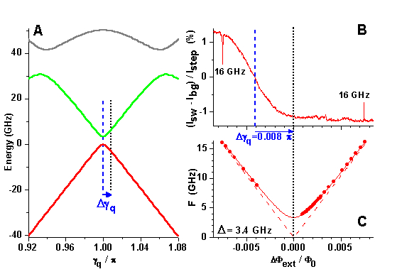
Fig. 4 (A) Qubit energy diagram (the first three levels). Around γq∼π, the qubit is a two-level system. (B) Ground-state transition step. A sharp peak and dip are induced by a long (1µs) MW burst at 16 GHz, allowing the symmetry point to be found (midpoint of the peak/dip positions, dotted line). (C) Frequency of the resonant peaks/dips (dots) versus the deviation in external flux from the symmetry point. The continuous line is a numerical fit (see (A)), leading to Δ≈3.4 GHz whereas the dashed line depicts the case Δ≈0.
Coherent oscillations
Next, we used different MW pulse sequences to induce coherent quantum dynamics of the qubit in the time domain. For a given level separation E10, a short resonant MW pulse of variable length with frequency F = E10 was applied. Together with the MW amplitude, the pulse length defines the relative occupancy of the ground and excited state. Corresponding switching probability was measured with a fixed bias current pulse amplitude (as explained above, we adjust Ib between the Isw0,1 values). We obtained coherent Rabi oscillations of the qubit circulating current for a frequency F = 6.6 GHz and three different values of the MW power A (Fig. 5). The variation in switching probability is around 60%, indicating that the resolution in a single readout is of that order. By varying A, we verified the linear dependence of the Rabi frequency on the MW amplitude, a key signature of the Rabi process (Fig. 5B). The oscillation pattern can be fitted to a damped sinusoid. For relatively strong driving (Rabi period below 10 ns), decay times τRabi up to ~150 ns are obtained. This large decay time resulted in hundreds of coherent oscillations at large microwave power. The Rabi scheme also allows the study of the state occupancy relaxation, by applying a coherent π pulse for full rotation of the qubit into the excited state and varying the delay time before readout. Experiments performed at F=5.71 GHz gave an exponential decay with relaxation time τrelax≈900 ns.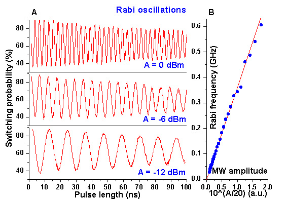
Fig. 5 (A) Rabi oscillations for a resonant frequency F=6.6 GHz and three different MW powers. The decay time of the oscillations is ∼150 ns. (B) Linear dependence of the Rabi frequency on the MW amplitude.
As a next step we measured the undriven, free-evolution dephasing time τφ, by performing a Ramsey interference experiment as follows. Two π/2 pulses, whose length is determined from the Rabi precession presented above, are applied to the qubit. The first pulse creates a superposition of the |0> and |1> states. If the microwave frequency is detuned by δF = E10-F away from resonance, the superposition phase increases with a rate 2πδF, in the frame rotating with the MW frequency F. After a varying delay time, we apply a second π/2 pulse to measure the final |0> and |1> state occupancy via the switching probability. The readout shows Ramsey fringes with a period 1/δF, as in Fig. 6A where E10 = 5.71 GHz, the microwave power A=0 dBm and δF = 220 MHz. The dots represent experimental data, whereas the continuous line is an exponentially damped sinusoidal fitting curve, yielding a free-evolution dephasing time τφ≈20 ns. Note that the oscillation period of 4.5 ns agrees well with 1/δF.
Additional information on the spectral properties of the decohering fluctuations can be obtained with a modified Ramsey experiment. By inserting a π pulse between the two π/2 pulses (Fig. 6B), we obtain a spin-echo pulse configuration. The role of the π pulse is to reverse the noise-driven diffusion of the qubit phase at the midpoint in time of the free evolution. Dephasing due to fluctuations of lower frequencies should be cancelled by their opposite influence before and after the π pulse. Spin-echo oscillations shown in Fig. 6B are taken under the same conditions as the Ramsey fringes, but here recorded as a function of the π pulse position. The period (∼2.3 ns) is half that of the Ramsey-interference. We measured the decay of the maximum spin-echo signal (i.e. with the π pulse in the center) versus the delay time between the two π/2 pulses. The data can be fitted to a half-Gaussian (not shown) with a decay time τecho≈30 ns.
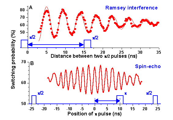
Fig. 6 (A) Ramsey interference: switching probability (dots) v. the time between the two π/2 pulses. A fit by exponentially damped oscillations (continuous line) leads to a decay time of 20 ns. (B) Spin-echo: switching probability v. the position of the π pulse. The decay of the maximum spin-echo signal v. the delay between the two π/2 pulses gives τecho≈30 ns.
[ note on the qubit operation:
we were not able to operate the qubit at the symmetry point which explaines the relatively short decoherence time in this experiment. In this device, the value of the tunneling gap Δ was rather close to the SQUID plasma frequency designed to be ∼2 GHz. This could be a possible explanation for the absence of coherent oscillations for F=Δ. ]
Conclusion
These first results on the coherent time evolution of a flux qubit are very promising. The already high fidelity of qubit excitation and readout can no doubt be improved. It is also quite likely possible to reduce the dephasing rate. Taken together, these results establish the superconducting flux qubit as an attractive candidate for solid-state quantum computing.[note for the reader:
The results presented here are published in Science, 299, 1871 (2003). For additional readings please refer to the refs. therein. ]